PCA stands for Principal Component Analysis. It’s what’s called an unsupervised learning algorithm and it’s a (clever!) way of reducing the number of dimensions in a data set. As a bonus, it reveals correlations between features.

As I was writing this blog post, I realized it was taking a very long time to make sure I have everything right, and it was getting really long, too, so I broke this post into two posts. In this first post I want to explain the idea of PCA and the math behind it, and then in the next post I want to talk about how I used it in my project and list some additional questions I have about it.

Most of my understanding of PCA comes from Matt’s data science bootcamp lecture on the topic. For this post, where I try to explain things in my own words, I’m assuming the reader has a very basic background in statistics (mainly voabulary words) and linear algebra (a first course).

The idea

Most data sets in practice have a very large number of features, and it’s impossible to graph them when there are more than 3. PCA resets the coordinate system so that only a few of the new coordinate vectors are needed to capture most of the variance in the data, while the rest of the new coordinate vectors have contributions that are small enough that they can be “flattened” (eliminated). This is useful when running supervised learning algorithms on the data, since fewer dimensions make the algorithms run faster.

Here’s the idea: Say you have a matrix of data, where the columns are indexed by the features of a data set and the rows give the observations for each feature. PCA turns that matrix into an ordered list of vectors. The first vector points in the direction of the highest amount of variance in the data, the second vector points in the direction of the highest amount of variance, out of all of the vectors that are perpendicular to the first. The third vector points in the direction of the highest amount of variance out of all the vectors perpendicular to both the first and the second, and so on. The vectors are the PCA components. Each component has an “explained variance ratio”, ordered from greatest to least, and so we can safely drop most of the components when the first few explained variance ratios add up to close to 100%.

The following visualizations are from Matt’s data science bootcamp lecture on PCA from fall 2022. The first visualization is a data set with two features, $x_1$ and $x_2$. The arrows on the graph are the PCA components, scaled so that their magnitude matches the variance of the data in that direction. The second visualization is the data replotted with the new coordinate system given by the PCA components. The point is that the variance in the data from the first graph is preserved in the second graph, the data points have just been rotated to make a more homogeneous picture.

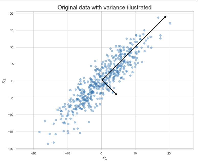
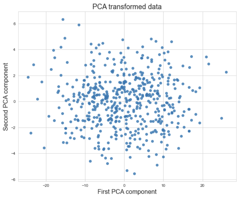
Now that we can see the highest amount of variance in the first graph spread horizontally in the second graph, the data points in the second graph can be flattened to the $x$-axis without losing much information about the variance. Flattening reduces this data set with 2 dimensions to one with 1 dimension.

The math

The problem PCA solves is an optimization problem. Let $X$ be the $m\times n$ matrix whose columns are vectors $X_1,\dots,X_n$ corresponding to the features. Each vector $X_i$ is $m\times 1$, and the entries are the observations of that feature. We wish to find a projection of the feature vectors to a vector $\vec w$, that has maximum variance, in other words, we want to maximize Var$(X\vec w)$.

To make this problem simpler, it is typical to scale $X_1,\dots,X_n$ so that they have expectation $0$. We also impose the convention that $||\vec w||=1$. Then the problem reduces to maximizing

\[\text{Var}(X\vec w) = \text{E}(\vec w^TX^TX\vec w) = \vec w^T\text{E}(X^TX)\vec w.\]

E$(X^TX)$ is just the covariance matrix!

It turns out the problem of maximizing any quadratic form $\vec x^TA\vec x$, where $A$ is a symmetric matrix and $||\vec x||=1$, is a standard problem in linear algebra called the constrained optimization problem. The solution is well-known (though not obvious, it’s a theorem). It’s the eigenvector of $A$ corresponding to the highest eigenvalue, and that eigenvalue is the maximum value attained by the quadratic form.

But what about the second highest value attained? If we impose the constraint that the second PCA component is orthogonal to the first one and of unit length (so we don’t distort our data with the change of coordinates), then we have another theorem in linear algebra that says the second highest value attained is the second highest eigenvalue. And it continues this way to get the next highest value, etc.

For each PCA component $\vec w$, the variance Var$(X\vec w)$ is called the explained variance, and is usually normalized as a percentage of the original variance Var$(X)$, called the explained variance ratio. It only takes the first few PCA components’ worth of explained variance ratios to add up to close to 100%, and so we lose little information about the data by throwing out the other PCA components. This is where the dimension reduction takes place.

Note: The vectors $X\vec w$, where $\vec w$ is a PCA component, are linear combinations of the features vectors. If some features are on a larger scale than others, then they will be overrepresented in the vectors $X\vec w$. For this reason, the features should be put on the same scale before running the algorithm in order to capture the true nature of the data.

For a more practical application of PCA in the NBA, see Matt’s blog post on the subject!